Pitchfork trading, multi-time frame and the scaling factor

This is going to be an important lesson for your perusal. Please take time to read it carefully, it contains essential information to increase your trading efficiency.

We want to discuss today how to trade with pitchforks in multi-time frame (MTF) environment. But before all, one must understand why we are doing it. It is not a matter of confirmation higher / lower time frame, it is not a matter of being more comfortable pending on your personal constraints, it is about decreasing risk and increasing profitability!

Before we dive into the pitchfork trading, let’s understand MTF risk reduction strategy and how we can decrease the risk by scaling DOWN and increase profitability by scaling UP !

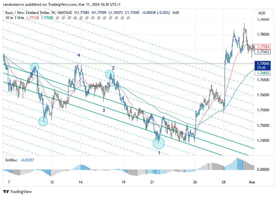
For this lesson, we are going to trade EURNZD. Let’s look at this recent price action on the 1-hour graph:

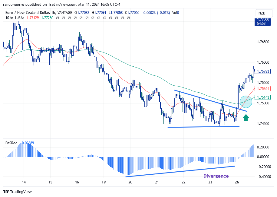
We have two moving averages, 25 and 100 EMA’s, and a smooth ROC indicator which does not care too much about which EMA you enter as a parameter. You have of course noticed a divergence with the ROC. You have even have drawn a kind of triangle of which escape yields a buy signal. However the red short term EMA is lower than the long one, so you may want to wait for a last confirmation with the crossing. Then you enter a trade, stop loss (SL) below recent low and target a 2.5 risk reward ratio (for instance):

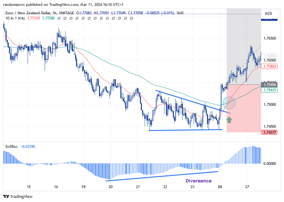
Your risk is 1.75456 (entry price) – 1.74377 (SL) = 0.01079 NZD

Can we do better?

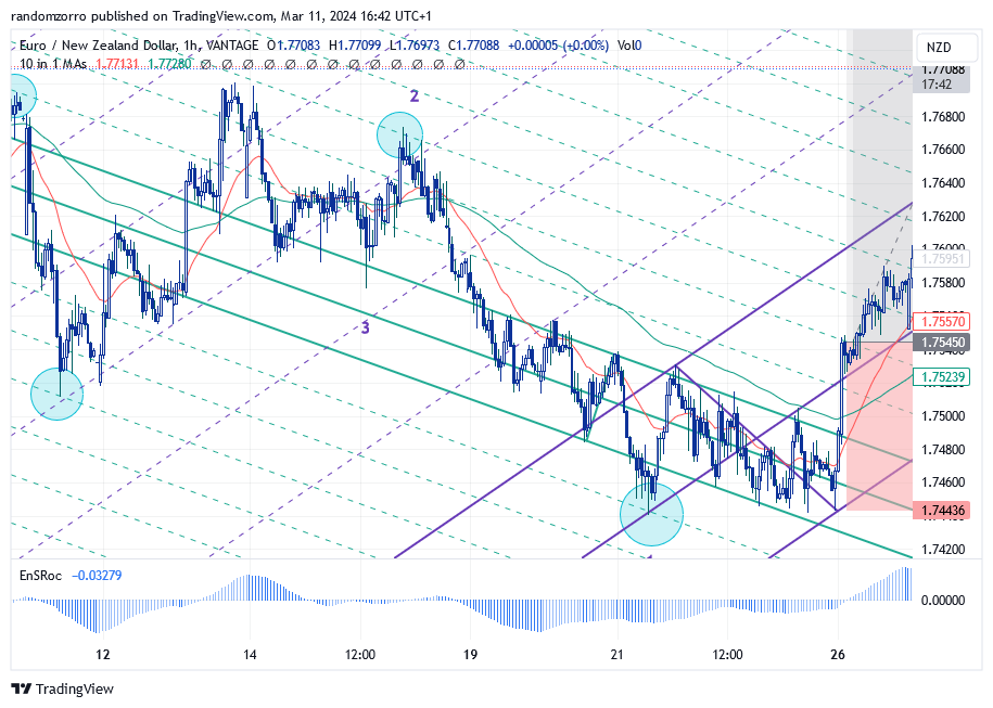
Let’s scale down to 15 min, meaning we switch the time frame of our trading software to 15 minutes. Same triangle but of course the moving averages have changed and the crossing is done when we exit the triangle! Momentum is positive and increasing. So nice!

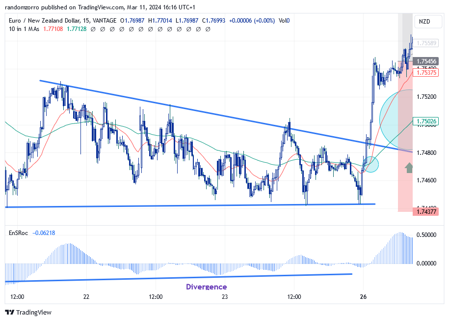
So I can place an order on this time frame.

I keep the same target price and stop as before, but I have managed to enter at a much better price, and my RR is enhanced from 2.5 to 5.22! For 10$ risk, I might earn 52.20$ instead of 25$, more than double my profitability.

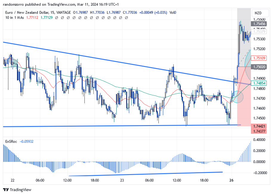
What about risk? Risk is now 1.75020 (entry price) – 1.74377 (SL) = 0.00643NZD, therefore a 41% risk decrease!!!!!

How did the trade go? Perfectly!

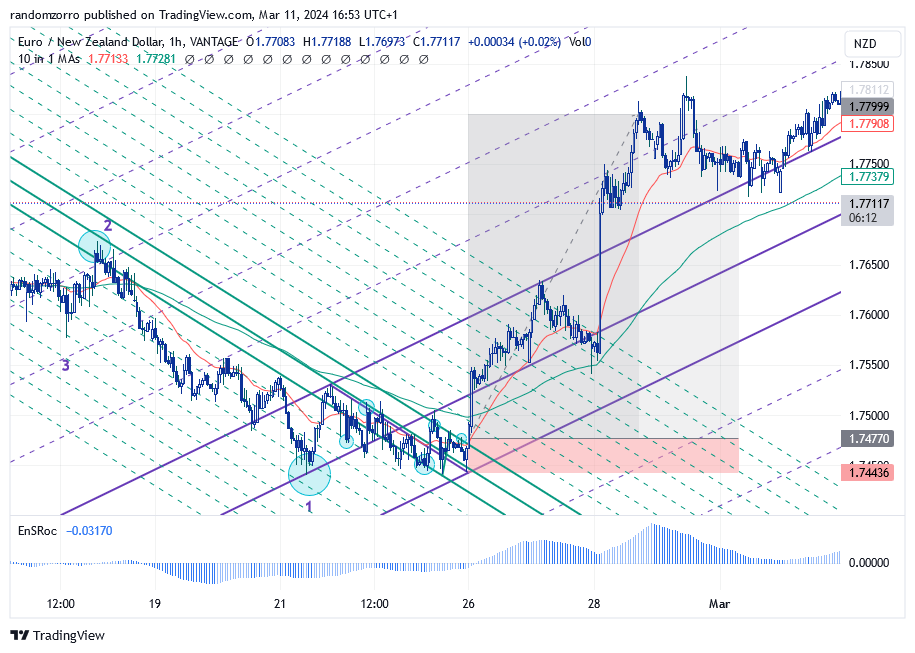
How does this relate to pitchfork trading? As you may remember, pitchfork gives us some sweat as we need to identify market structure, take the pitchfork, which may work or not during validation. So we don’t want to draw it on 1 minute charts! For the trade above, let’s see what can be done

Market structure is obviously a down trending one, but the mini-pitchfork did not make me comfortable so I had to hybrid it (more on that in future posts). Now I have multiple contacts with warning lines. I feel better and I see prices exiting the pitchfork at the same timing, more or less.

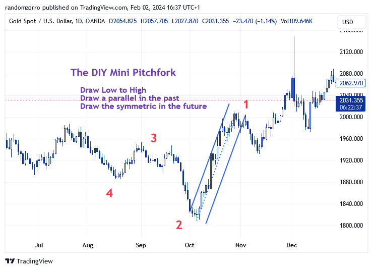
Now you can draw a new pitchfork as SP1 is fully confirm to be a local trough, and a SL can be placed below the lower MLH:

You can of course move your SL along the lower MLH to make a trailing stop!

Your risk is 1.75450 – 1.74436 = 0.01014 NZD

Can we improve?

Well yes! We can keep the purple pitchfork but on 15 minutes, you need to find a new trigger pitchfork (green one) with new market structure at that level:

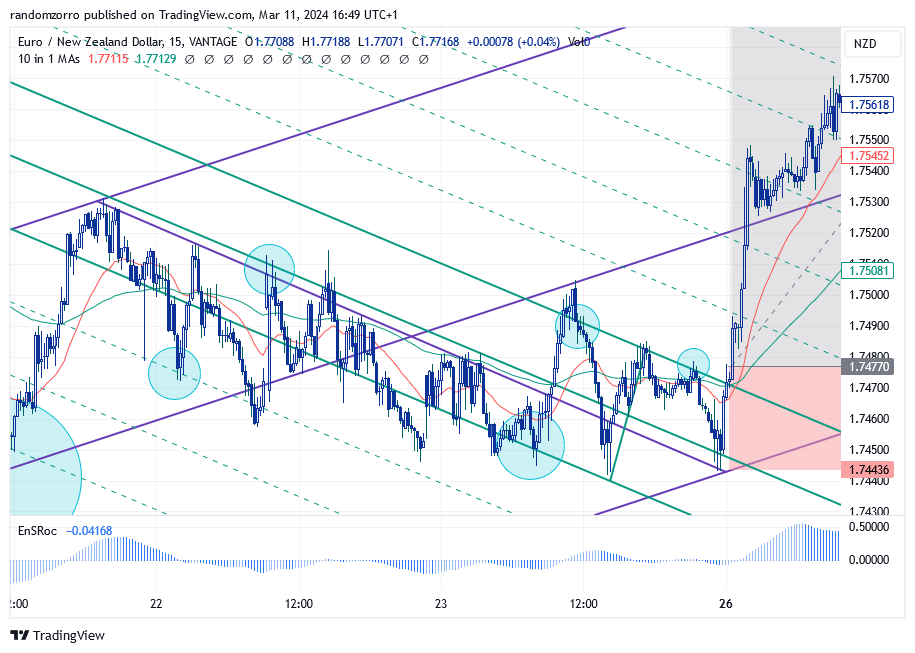
Place buy order on top of the exit candle. Now your RR has hiked from 2.5 to 9.57!!!!

Your new risk is 1.74770 – 1.74436 = 0.00334 NZD so a 77% risk reduction.

Of course same trade turned out the same

Whatever trading system you use, you can get the same benefit from scaling down.

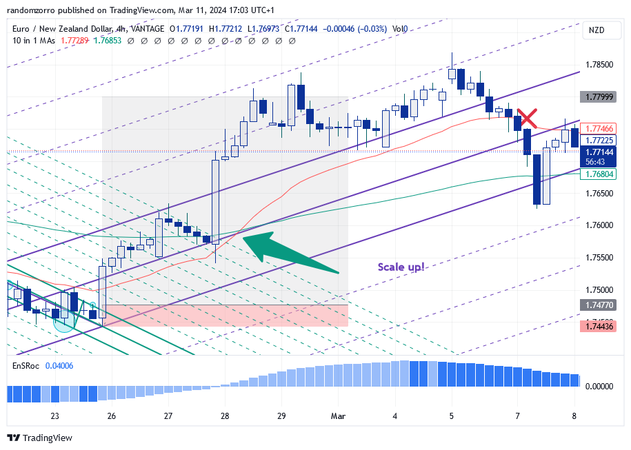
Now let’s look benefit of scaling up:

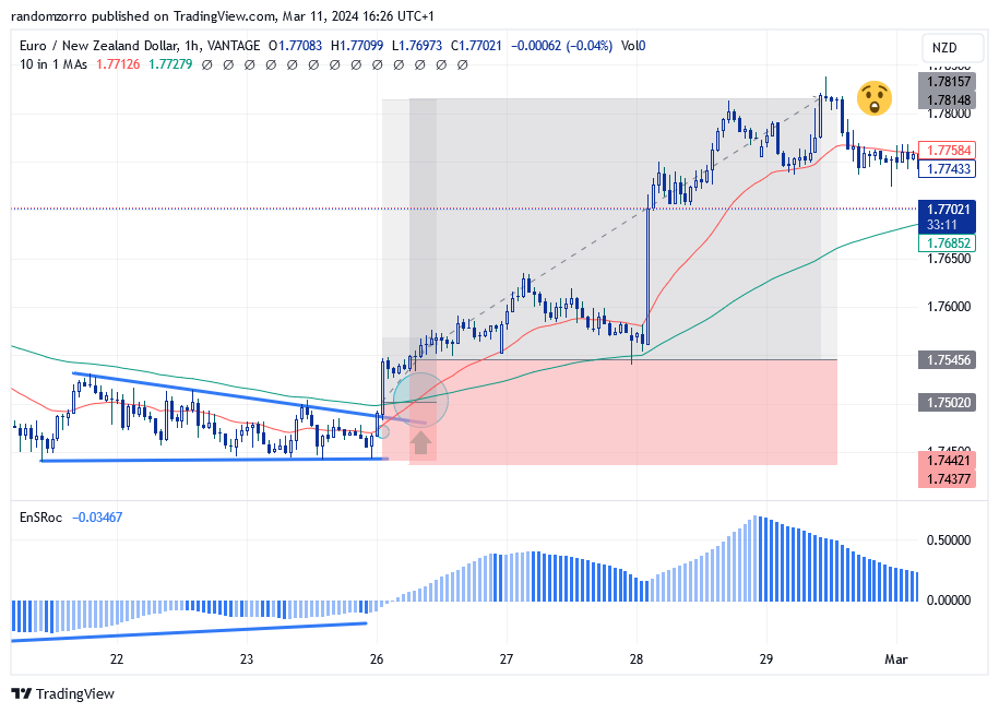
On the 4h time frame, once we get a similar golden cross between the short and long EMA’s, we are allowed to scale up:

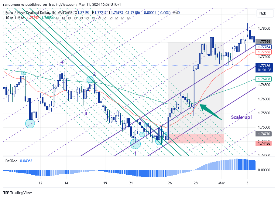
After the golden cross, your trade is hugely profitable, so you want to secure some profit. For the remaining of the line, you may want to target extra profits. Place your trailing stop below the red average for instance and let your profits run for as long as the market wants.

In this particular case, it did not work but my RR was around 8.

That’s it for today. The example was with forex today but it is of possible to use this strategy on 5min/1min time frame or on crypto and you could get huge RR’s (>30) from time to time. Enjoy.

And until next time, trade safely!

Market structures transitions. Introduction about mini pitchforks

I hope you had some thoughts about the market structures, how they are built and you understand why there is no need to have more figures. Each structure requires the use of specific pitchfork for an efficient trading. But first solution to the proposed exercice. I hope you had fun and did some drawing on a table, result should look like that:

On second thought, there may some transitions missing here. I will let you find out…

There are a few points to remember from this study:

  • When market is is consolidation mode, it can consolidate even more (the circling back for bottom figure)
  • A trending market can move into consolidation without notice
  • Reversal structures don’t end up in flat market

Let’s move now to mini pitchfork subject. On the following gold chart, I selected 4 swing points that describe an unstable market. If you refer to previous post, I can use a mini-pitchfork to get a buy signal.

As you can see, I have selected minor peaks and troughs on the path from SP2 to SP1. I can’t say it is the most relevant choice but if you look at warning lines, prices are indeed stopped or pause before continuing their path.

On the following example, it is not so obvious, but I used the extreme price at the end of wicks to create my pitchfork. An other way to trace it is going down to lower time frame so you get bigger waves….

Sometimes it is not possible to identify minor peaks or troughs, so we work it out manually. You may draw warning or you can attemps using the pitchfork tool to overlay your DIY pitchfork: select first SP on the HL line, take SP2 on upper line, and SP3 on lower line and it should do the trick

The way to use mini pitchfork is similar to other pitchfork. We will see many examples in future posts.

Until then, trade safely.

Being in Bitcoin awesome bull market!

As written a few times, social network are stealing your time, your data, your ideas, and everything else they can. As of now, they tell who can tweet or put message on Facebook, they can remove any content they don’t like, … No surprise either when some say “Bitcoin is a worldwide scam”. It may be somehow, Bitcoin have no greater reality than fiat moneys, as their names indicate, but for traders in the short term, Bitcoin exists and the risk is just a bit bigger because of volatility. So it is worth having a strategy to enter at low volatility levels and decrease exposure when volatility is too high to your taste. If you don’t have or don’t want to spend too much time with custom indicators, just draw the infamous Bollinger bands and a long term MACD (parameter 48 and 64 for instance) on any financial web site as below:

MACD is positive, so the long term trend is up. No further question to be asked.

You can also see areas where those bands are getting closer to each other. Change the Bollinger moving average to 5 or 7 days if not visible enough.

Then if you compare where we are compared to previous bull run, as indicated with green smileys, we are barely at the beginning of ‘second phase’ of Bollinger bands, indicating the strong bull market will continue, albeit most likely on a quieter pace.

To get a peace of mind, consider the difference between last price and green moving average. That is your risk! If too far away (consider how many $ or € you could loose), just decrease the position size, thereby also securing some of the profits!

That’s it! Until next time, trade safely!

Portfolio management – the myth of diversification

Continuing the myth busting series, we have now to challenge the way we are proposed to manage a stock or any securities portfolio.

Why are we supposed to diversify our portfolio? Finance people tell us that market is unpredictable, stocks go up and down and having a balanced portfolio allows to prevent wild swings for your money. Think about it for a moment!

Sorry guys, most people want to know how to go from A to B, I can’t guide you!

If some stocks go up and some go down, how performant is your portfolio going to be? Very average! A performance close to zero is probably what they expect you to do. Now you have an objective which is making as much money as you can (don’ t lie!) while having not too much stress, so let’s study the ‘one-stock portfolio’!

This strategy is actually a diversification kind of portfolio, but instead of using stocks from different sectors, … we will use time diversification for a single stocks. How does it work? Easy! Consider a stock for which the long term trend is up, for which you know there a sunny future, … Could be some AI, robotics, cannabis(?), …

Let’s consider Adobe Systems for the example. Adobe makes multimedia and creativity software products, digital marketing software. Adobe is also known for its Adobe Flash web software ecosystem, Photoshop image editing software, Adobe Illustrator vector graphics editor, Acrobat Reader, the Portable Document Format (PDF), … A long history of innovation and most likely a brilliant future ahead.

First step: Let’s look at the monthly chart:

Trend has been up for very long time, I do not advise to invest right now, but you see the idea. Start investing the first day of a month a number of stocks that matches your risk sensibility. See previous blog posts here or here . Beginning of next month, check where market is and how much money you still have at risk. If stop has gone up, voiding your risk, add extra stocks so you still have x$ at risk for the following month. You are accumulating by averaging up!

Second step: we diversify with the weekly chart.

We are closer to trading now. Add additional stocks to your portfolio when your trend indicator (a MACD in our example) confirms the price crossing over the red stop line. Use same criteria for line sizing! Exit those specific line when indicator crosses down its signal (don’t wait for the stop!)

Third step: we are going to boost the performance by trading the daily chart. Ideally you want to do that with CALL and PUT options, while considering your risk is 100%, should you misinterpret your chart.

You need to check momentum and volatility before entering your position. You need to master of course option trading, idea is of course to use here rather long term options. Exit when any of the indicator tells you to go out (stop or momentum or volatility). You may also use a stop much closer to the prices. When trading the down side, you are also covering for the down swings of your monthly positions so don’t expect huge gains these months, you are therefore also achieving portfolio volatility control via time diversification!

We like very much this strategy. We advise you to test it in details before trying it out for your portfolio. It does not work with all stocks. The dividends collected part of weekly and monthly lines are of course re-invested.

Note we have had this Adobe stock portfolio for real for the last 10 years. The yearly performance has gone to the 3-digits area a few times!

That’s it. Until next time, trade safely!

Have you been fooled by the bell curve?

I know you like some food for the mind for the week-end, this post is sure to make you think even it is simple mathematics! Of course, it will be fun to read too!

I have talked previously about how not use the Bollinger bands and I am going to kick even more on this concept.

As soon as you start talking about standard deviation (or sigma), you are assuming a bell curve, that is 62% of measurements (price) should be within one standard deviation of the average price. Let’s check that immediately, let’s display a Bollinger band with 1 sigma on Apple graph:

Apple Daily

Now look in each blue blox. There is almost ZERO price inside the band! The guy who sold the Gaussian curve to finance was the best salesman EVER!

Though attributed to Gauss, the bell curve was created by Abraham de Moivre in 18th century and then promoted furiously by an Adolphe Quételet in 19th century. Johann Carl Friedrich Gauss, one of best ever mathematician, published a book about normal distribution for astronomical data, and since then, we are talking the Gaussian or bell-shaped curve.

Gauss never studied the stock market random data! And standard deviation is only a ‘trick’ to locate 62% of the data around the average.

As shown on Apple graph, stock data is not consistent with normal distribution. Now what? When you have spotted a problem in trading, you got an edge!

You may remember from your years in high school the basic average deviation, sometimes called mean absolute deviation (MAD). In other words, it is the raw deviation measurement. Quoting Wikipedia:

MAD has been proposed to be used in place of standard deviation since it corresponds better to real life.[3] Because the MAD is a simpler measure of variability than the standard deviation, it can be useful in school teaching.[4][5]

School teaching? Hmmm… Most important part is first sentence: it corresponds better to real life! More on the difference between MAD and Gaussian distribution by fabulous Nassim Taleb here.

Stock price is not an industrial process measurement, it reflects the opinion of all people about the studied stock. If you are a car manufacturer and making 4.50m long cars, your production should make cars, say between 4.49 and 4.52, because otherwise the doors will not close properly is car is 4.78m long and you will need re-manufacturing with all associated costs! That is not the case for stock price, you are allowed to be excessively bullish or bearish!

Let’s give this theory a try. I am removing the Bollinger bands and adding a simple moving average, 34-days for the example, but you may change it.

Steven Nison, in his book introduced the Disparity indicator, created by Japanese traders, which is defined by:

Disparity = close – average over n days of close

It is very close to what we are looking for! We only need to add an average to get the Moving Averaged Disparity (MAD also just to add confusion!)

Apple Daily

The blue line is disparity and the MAD line is shown green when pointing up, red when pointing down.

As you can see, trading is almost straightforward. Buy when prices are over the 34-day average and disparity crosses over MAD (or when price cross over average and disparity is above MAD). Then get out when prices drop below average! Easy, isn’t it? You also get some nice divergence at the top, disparity has crossed below MAD end of January, far before the correction started!

From this introduction, there are plenty of ways you can improve this very basic but nonetheless very efficient indicator!

Here is a non commented graph of Nasdaq for you to play with:

That’s it! Until next time, trade safely!

Volatility lovers: Crypto, what else?

Investing in crypto currencies might be something for geeks, many of you probably think, but for the pleasure of trading small amounts and and making big gains in percentage, this is worth a detour.

It is not because you hate some companies that you should not invest in them. Trading is about making profits, full stop. Yes, crypto may not environment friendly, and will be worth zero should a huge wordly power outage occurs but that is a risk you have to manage. Also crypto are showing the path to the future, nobody in maybe 10 years from now will pay with banknotes and coins. This is why you should be bullish on this technologies and why not trade of few them!

There is now a big number of cryptocurrencies to invest in, but please stick to major ones, as most of them are scams and will be worth zero far before our gigantic power outage! I do not wander beyond the big ones like Bitcoin, Etherum, Litecoin and a few others. Trading those is actually quite straightforward because of huge volatility, and remember volatility means also likeliness of emergence of trends. Use a Kagi graph to enter is easiest strategy, then use a candlestick graph to place stop!

Here we go with Bitcoin!

Bitcoin bottomed out by March 22nd, Kagi lines made a 2-level break, MACD is up. One day later, the double window bottom was also confirmed. I entered below 6000!

If the accumulation/distribution also showed a buy signal about the same time, it was not so obvious we should go! Skeptic bull, uh? As the trend lines then started going up beginning of April and price starting to hover the random walk path, it was second possible entry!

Where is Bitcoin headed now? As you can see on Kagi, the Bollinger bands are pointing upwards. A correction may or may not come, next objectives are 10700 and 12000. Out if closing below 8800 (as of today!). Just wait and see!

Note: major crypto currencies will not disappear tomorrow, unless this enormous power outage again! Using a stop based on volatility is fine. But price may zoom through the stop line, so be careful and make the line size much smaller than on a stock and you will be safe!

Three-Line-Break or the integrated trend-volatility tool

I have been a fan of Three-Line-Break (TLB) trading for long time because it is a KISS (Keep it Simple Stupid) methodology and takes no time to make decisions, which is mandatory when you have an other full time job! As long as I did not have any backtesting tool and was working only small caps which are trending usually for longer period of time, then the feeling was there was a positive expectancy. However, from time to time, I experienced losses more than I liked, and felt like missing trend departures.

Once again I assume you are already knowledgeable about the basic topic. For more details on TLB, please refer to here

Backtesting becomes possible when you can actually display the TLB back on daily chart. On the following chart, you can see on the right the TLB chart, with red and green lines; these appear on the left candlestick chart as red and green boxes.

There are signals from TLB that you would obviously not take after adding our usual 3 single Moving Averages for instance.

When we backtest over long period of time the TLB strategy on standalone only, we surely are disappointed.

Let’s look at Apple. First with TLB, taking buy and short signals, 300%

Taking our 3-moving averages on the long side only, we fare far better!

So if you hate candlestick charts, then you need to put those 2 technologies together. First add the 9 and 18 averages on on your TLB chart.

The size of each TLB line represents also the volatility, though you don’t know how long it took to have this volatility increment. Fair enough, the daily volatility is filtered out to show the trend volatility. The ROC indicator should be very talkative. I am displaying the ROC 9 days on this chart:

Any time, ROC crosses 0, or just touch down 0 and goes back up are good entry points. When ROC is positive, just filter out the short signals. An other confirmation is SMA9 is above the SMA18. And there are also divergences to help anticipate trend change!

You may also look at the volatility of 3LB, this time using Bollinger bands, because TLB lines stick to 2 standard deviations!

I tried to move back these good-looking curves to candlestick charts for back-testing but to no avail. So I can not show you the backtesting result.

As a conclusion, if you are not after option trading where time does matter, these TLB chart are a very good tool. Overall trend is given by a single moving average, which allows easy filtering of false signals.

That’s it. Until next time, trade safely!

Spotting and trading the Random Walk path!

After discussing raw volatility, standard deviations, no way we don’t have a discussion about ATR aka the Average True Range. This post will definitely blow you mind, I am going to demonstrate that markets are REALLY following a random walk path, pushing from one side to the other in a precise manner.

For introduction, please read again my previous post about drunkard’s walk.

Let’s consider an observation period of n days. The Highest High (HH) and Lowest Low (LL) may be considered as lamp post from which our drunken guy is walking. We know that on average we should be able to find him at a location situated at square root of n multiplied by average stride length or the Average True Range over n days to use financial wording.

Here is how it looks:

The red line is where Bulls expect price to be, whereas the Bears are waiting for the prices to reach the green lines. These are all average expectations of course, and these objective can be reached any time during the observation period. Please remember that down markets are usually twice faster that up markets.

What if we consider the middle price between these 2 expectations??

Let’s do a bit of maths:

  • Today’s high (H) is expected at LL + 2 * √n * ATR(n)
  • Today’s low (L) is expected at HH – + 2 * √n * ATR(n)

So the middle point can be defined as:

MP = .5 * ((H+L)/2 +(HH + LL)/2)

Of course price will not be there, X does NOT mark the spot, but it is a fair expectation about where prices should be, if there were no other information.

Let’s display it on a real chart!

We are going to use n = 36 in this post, you can use anything between 4 and 100, but make sure the square root is an integer for what will be following.

Ouch! It hurts the eyes. But you need to think of it differently. It is not a simple moving average, it is always using the most significant average of the day, between 1 and 36. Anyway you can already see that, when prices are above the path (light blue color),then trend is up. The path leaves a chance to prices to retrace and tends to be closer to them before a reversal.

Let’s not stop there and use a standard average of this path to smooth things out. Now follow my reasoning!

If the random walk theory holds, then the path we have spotted may very well be a lamp post so the actual prices should hover at exactly a number of strides from the lamp post, not 3.7 strides, 4 really! Let’s do it and display some lines at exactly every 2 steps (2 ATR’s) from the middle path.

Whaouh!!!!!!!!

The red/green line is the smoothed out path. Prices are pushing along the lines, see only a few examples highlighted in red circles here:

Just amazing.

One way to see it is to consider the middle path as the median line if you were using an Andrew pitchfork, first lines above and below are the MLH (median line high) and the other lines are warning lines!

Even better, if you are looking for warning lines above a major bottom, each represent a price objective. In the case below, the price identified on first warning line is reached a the top second red circle within .30$! (97.70 vs 97.42!)

Trading strategies are quite straightforward from then on:

  • From a warning line far below median path, play return to the path
  • From middle path that is going, play the trend and put a stop on a visible line below the price
  • If price is ‘in the central pitchfork’, most likely there is no trend!

Now, you will tell, this is an example, sure it does not work with last market conditions? Yes it does!

Here is Nasdaq recent price action, stopped on a warning line!

Or McDonald. Doing quite well!

Final thoughts: Market is moved by demand and offer. Behind these are drivers are humans or robots programmed by humans who can change their mind any time, giving the market a random outlook. This post would be worth many more investigations. Dr Andrew and his pitchfork really had a hint, but without computer, it was definitely more difficult for him. This is maybe the first explanation why Andrew Pitchfork are working and why it is so difficult to identify the right pivots to draw the pitchforks! Anyway, the random walk proves to a very good model, again because we are not trying to fit the data into a specific model or data distribution!

Feel free to comment or send email.

Until next time, trade safely!

Bollinger bands from a different perpective

As a blog about volatility, of course, there must be a post about Bollinger bands, which is the most common way to assess volatility. More especially, finance have based all their systems, assuming that prices are a Gaussian distribution (aka bell curve).

If this statement was true, then only 2.14% of prices should be outside the 2 standard deviations (aka sigmas). For one year, say 200 days, 4 days should be oversold or overbought, as commonly said!

Fair enough, let’s work a quick indicator that tells us how many sigmas the prices are from the average. We are taking John Bollinger’s definition.

Indicator = (close – 20-days average of closing prices) / Standard deviation 20 days

Let’s look again at Apple graph over last few months!

We have gone beyond the 2 standard deviation at least 8 times, sometimes for a few days. It is not looking good! If you are looking at S&P500, it reaches -3 sigmas once a year at least, when it should be the case more or less once every 8 years. Of course, it is probabilities, and this can happen more often. Correct, but there should be also long years without this far reaching. Which is not the case!

Now that you have spotted this interesting paradox, you have a new edge for trading! The best to trade Bollinger bands is just to NOT draw them. Remember that bubbles and parallels pointed by by Bollinger specialists are mere illusions!

Instead use our small indicator!

The indicator displays many divergences:

  • Blue ones are standard divergences with the price to spot reversal
  • Green ones show hidden divergences in the direction of the trend

I have highlighted a red one to show one that did not work. Be careful, if the trend is strong, wait for a signal to profit by the divergence, at least let the price go over the short moving average.

See, it is easy! For standard divergences, make sure first point is in oversold or overbought area, as indicated by the 2 sigmas lines.

One you are in, don’t get out of your trade at the 20-days moving average (strategy called ‘return to mean’), use a trailing stop, the green average for instance.

That’s it. Some people would charge you 5000$ per year to then send you the signals by email. If you do sell this service, please remember my commission!

Volatility Trading System superior performance

I wrote in some previous posts that volatility trading improves the performance of any trading system. Is it the case? Really? How better is it?

The goal of volatility analysis is to get rid of loosing trades as much as possible, so if you go from 30% winning rate to 60%, then number of consecutive loosing trades will be narrowed down, the overall profitability will increase.

Let’s start this demonstration with a simple yet very interesting trading system:

  1. Buy when close > SMA(9)(close) > SMA(18)(close) > SMA(50)(close)
  2. Get out of the market when close is crossing under the SMA9

Close is today’s closing price, so you buy at the opening the next day. SMA(x) are x days simple moving averages. I am not taking short positions for this exercice, the rules would be exactly opposite.

Here is the graph of Apple over last few months. The 3 moving averages are shown by red (9 days), green (18 days) and blue (50 days) color. Some entries are shown with green arrows and selling the position by red crosses.

Looks good, doesn’t it? As long as the stock is capable to trend and Apple perfectly fits this criteria, this trend trading system should be ok.

Let’s now run a systematic simulation for a portfolio (10k$) with only one line and re-invest 100% of the profits. Here is the result:

Over 20 years, you multiplied your capital by 8! Great 🙂

But a few considerations are needed:

  • A buy&hold strategy would have yielded much more (x18)
  • you get 35% winning trades, a win/loss ratio of 1.67, biggest gain is 14257$, largest loss is 6226$
  • As expected from calculation in previous post, we can get a series 12 loosing trades in a row

Psychologically it is tough to handle, but could be worse. If you traded Cisco instead of Apple, the result is negative! That is because volatility is not big enough!

Now if you traded Bitcoin with this system, you are a billionaire! See the graph and report just below! Notice an almost 300M$ loosing trade, that is undoubtedly hard on the psychology!

Now I am adding volatility control on Apple, on top of previous one:

See? Now we multiply our initial capital by 41 (started from 100k$), beating by far buy&hold strategy! Now we get 68% winning trades, a win/loss ratio of 3.77, max 7 consecutive loosing trades but 16 long series winning trades 🙂

That’s it for today! Until next time, trade safely!